Measuring the SALSA antenna beam
Based on earlier work by Eskil Varenius, Onsala Space Observatory

Every radio telescope has a characteristic beam — a description of how sensitive it is in different directions on the sky. Knowing the beam shape is essential for interpreting any measurement made with the telescope. In this experiment, you use the Sun as a bright radio source to map the beam of SALSA directly, by measuring how the received power changes as the telescope is pointed progressively further away from the Sun.
The Sun is an ideal calibration source for this purpose: it is far brighter than the background sky at radio wavelengths, it is small enough relative to SALSA's beam to act as a point source, and the telescope can track it automatically. A set of short measurements at different angular offsets is all that is needed to trace out the beam profile.
Note: this guide focuses on the theory and scientific interpretation. Instructions for operating the telescope can be found in the User's manual.
1. The radio telescope beam
1.1 Angular resolution
Any optical instrument — a camera lens, a pair of binoculars, or a telescope — can only separate two nearby objects on the sky if they are more than some minimum angle apart. This minimum angle is the angular resolution of the instrument, and it is ultimately set by the wave nature of light through a phenomenon called diffraction.
When waves pass through a circular opening of diameter D, they spread out by diffraction. The smaller the opening relative to the wavelength λ, the more the waves spread, and the worse the angular resolution. The Rayleigh criterion gives the minimum resolvable angle as:
θ ≈ 1.22 λ / D
where θ is in radians, λ is the observing wavelength, and D is the aperture diameter. A larger telescope or a shorter wavelength gives better (smaller) angular resolution.
Radio telescopes observe at much longer wavelengths than optical telescopes — centimetres or metres rather than hundreds of nanometres. This means that to achieve the same angular resolution, a radio telescope must be vastly larger. SALSA's dish is 2.3 m in diameter, and it observes near 1420 MHz (λ ≈ 21 cm). Applying the formula:
θ ≈ 1.22 × 0.21 m / 2.3 m ≈ 0.11 rad ≈ 6°
So SALSA can only distinguish features separated by about 5–6° on the sky. This is quite coarse by optical standards — the full Moon is only 0.5° across — but it is sufficient to map the large-scale structure of the Milky Way's hydrogen emission, as in the HI experiment.
1.2 The beam of a circular aperture
The antenna beam (or beam pattern, or response function) is a complete description of the telescope's sensitivity as a function of direction. It is not simply a sharp cutoff at the angular resolution limit — instead it has a smooth main lobe with a peak at the pointing direction, falling off on either side, and a series of smaller sidelobes at larger angles.
For a uniformly illuminated circular aperture, the beam pattern is an Airy function — the same pattern seen in optics when light passes through a circular hole. In the central region the beam closely resembles a Gaussian, and the full width at half maximum (FWHM) is:
FWHM ≈ 1.02 λ / D
Note that the related Rayleigh criterion (θ ≈ 1.22 λ/D) gives the angle to the first null of the Airy pattern, traditionally used as the resolution limit for separating two point sources. The FWHM is about 16% smaller — a more direct measure of the beam width itself.
For SALSA at 1408 MHz (λ = 21.3 cm) this gives FWHM ≈ 1.02 × 0.213 / 2.3 ≈ 0.094 rad ≈ 5.4°.
Beyond the main lobe, the Airy pattern has sidelobes at roughly 1.7%, 0.4%, and 0.2% of the peak sensitivity. Although small in relative terms, sidelobes can pick up emission from directions far from where the telescope is nominally pointed, which is important to keep in mind when interpreting observations.
1.3 Why use the Sun?
To measure the beam we need a compact, bright radio source — ideally a point source much smaller than the beam, so that the measured response traces the beam shape directly rather than being blurred by the source's own extent.
The Sun is an excellent choice for SALSA for several reasons:
- Bright: The Sun is by far the strongest radio source in the sky accessible to SALSA — a short integration of just a few seconds gives a clear detection, making it practical to measure many offset positions without a long observing session.
- Small enough: The Sun's angular diameter is about 0.5°, which is much smaller than SALSA's ~5° beam. It is not a perfect point source, but small enough that it barely broadens the measured beam pattern.
- Easy to track: The Sun moves across the sky predictably, and SALSA can track it automatically — no coordinates need to be entered manually.
The main limitation is that the Sun is only observable during daytime, and the experiment requires the Sun to be well above the horizon.
2. Observing with SALSA
2.1 When to observe
This experiment requires the Sun to be above the horizon at Onsala, Sweden — so observations must be made during daytime. To get the strongest, cleanest signal, observe when the Sun is as high as possible in the sky. The Sun reaches its highest elevation around 11:00 UT (noon local Swedish time). Earlier or later times also work well, particularly during the long Swedish summer days. Avoid observing when the Sun is below about 15° elevation, as the signal becomes weaker and ground emission starts to contaminate the beam sidelobes.
You can check the Sun's current elevation using a planetarium app or website before booking your observation slot.
2.2 Tracking the Sun and offset positions
In the observe page, select Sun from the Target dropdown. SALSA will automatically calculate the Sun's position on the sky and track it — no coordinates need to be entered. Click Track and wait for the telescope to reach the Sun's position.
To map the beam you need to measure not only on the Sun itself, but also at a series of offset positions in different directions from the Sun. Use the Advanced tracking settings section to enter azimuth and elevation offsets in degrees. For example, entering an azimuth offset of +3° will point the telescope to a position 3° away from the Sun in azimuth.
A typical scan strategy is to hold the elevation offset at 0° and step the azimuth offset from −10° to +10° in steps of 0.5° or 1°, making one measurement at each position. This gives a one-dimensional cut through the beam. You can also scan in elevation, or make a two-dimensional grid to map the full beam shape.
Each time you want to change the offset, click Stop, enter the new offset values, and click Track again. Wait for the telescope to settle before starting the measurement.
Azimuth vs. elevation offsets: Elevation offsets directly equal the angular distance on the sky — a +2° elevation offset moves the pointing 2° up. Azimuth offsets behave differently: because lines of constant azimuth converge toward the zenith (just as lines of longitude converge at the poles), the actual angular separation on the sky is smaller than the entered value:
θ = cos(el) × Δaz
For example, if the Sun is at elevation 45°, an azimuth offset of +4° moves the pointing only cos(45°) × 4° ≈ 2.8° from the Sun on the sky. To achieve a spacing of 3° on the sky you would instead enter 3° / cos(45°) ≈ 4.2°. At the elevations typical for this experiment (roughly 20°–50°), the factor cos(el) ranges from about 0.64 to 0.94 — noticeable when comparing your measured beam width to the expected value.
2.3 Receiver settings
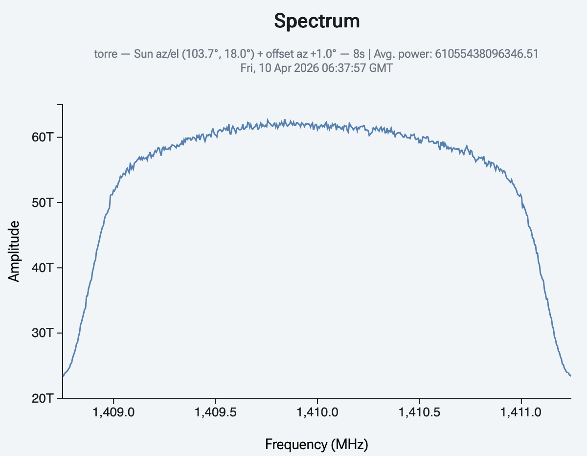
When you select Sun as the target, SALSA automatically switches to Raw mode, which measures total received power directly — exactly what is needed for this experiment. The default centre frequency is 1408 MHz with a bandwidth of 2.5 MHz. The Sun is very bright at radio wavelengths, so the narrow bandwidth gives a perfectly clear detection — just click Start and 1 second of integration is enough.
Keep the frequency at 1408 MHz rather than tuning to the hydrogen line at 1420.405 MHz. At 1420 MHz the receiver would also pick up 21 cm emission from neutral hydrogen gas in the Milky Way along the line of sight, which would add a varying background to your measurements and make it harder to isolate the Sun's contribution. At 1408 MHz you sit safely clear of the HI line and measure essentially only continuum emission from the Sun.
2.4 Measuring and recording power
For each offset position, click Start, wait a few seconds, then click Stop. The key quantity to record is the average power, shown in the chart subtitle as "Avg. power: …". This is the mean antenna temperature across the observed bandwidth, and it is what you will plot against the offset angle to get the beam pattern.
Keep a table of your measurements as you go, for example:
| Az. offset [°] | El. offset [°] | Avg. power |
|---|---|---|
| −10 | 0 | … |
| −9 | 0 | … |
| … | … | … |
| 0 | 0 | … |
| … | … | … |
| +10 | 0 | … |
A complete azimuth scan from −10° to +10° in 1° steps takes about 25 minutes including telescope slewing time. Plan your observation slot accordingly.
3. Analysing the beam
3.1 Plotting the beam pattern
Once you have a table of average power values at each offset, plot them: put the azimuth offset (in degrees) on the horizontal axis and the average power (in K) on the vertical axis. You can use any spreadsheet or plotting tool — LibreOffice Calc, Python with matplotlib, or similar.
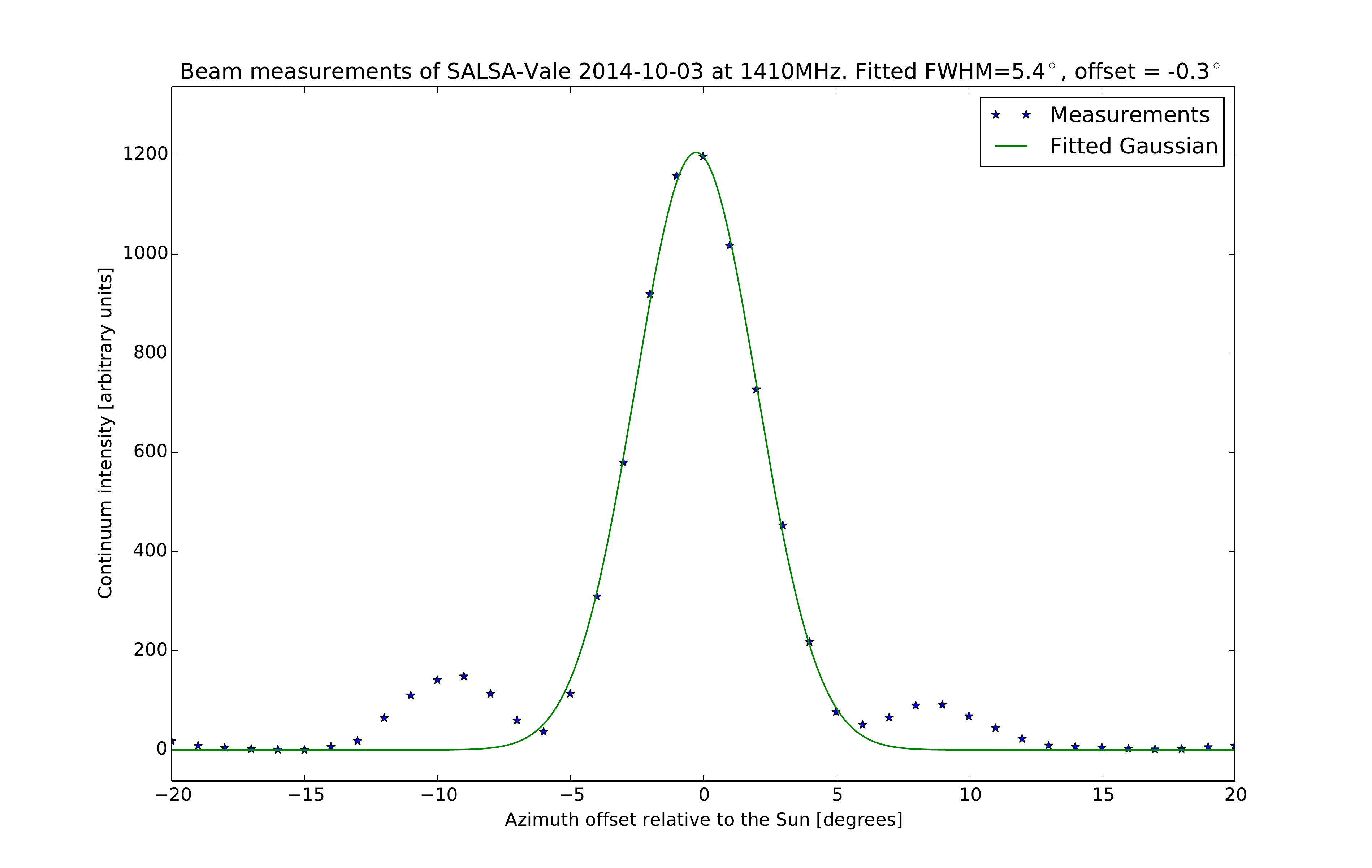
The result should show a clear central peak at offset 0° (the telescope pointed directly at the Sun) with the power falling off on both sides. If your scan extends far enough you should also see the sidelobes — smaller bumps at roughly ±8–10° from centre. Fig. 3.1 shows a measured beam from the SALSA telescope.
3.2 Measuring the beam width
The most important number to extract from the beam pattern is the full width at half maximum (FWHM) of the main lobe — the angular width of the beam measured at half the peak power.
Your measurements will include a non-zero baseline — the background sky power received even when the telescope is not pointing at the Sun. Before estimating the FWHM, subtract this baseline level from all your power values. A good estimate for the baseline is the average power measured at your largest offsets (e.g. ±10°), where the Sun contributes negligibly. Once subtracted, the peak at offset 0° represents the Sun's contribution alone.
To find the FWHM from your baseline-subtracted data:
- Find the peak power value (at offset 0°).
- Calculate half that value.
- Find the two offset angles where the measured power crosses the half-power level (one on each side of the peak).
- The FWHM is the difference between those two angles.
For a more precise estimate, fit a Gaussian curve to the main lobe. A Gaussian has the form:
P(θ) = P₀ × exp(−4 ln 2 × θ² / FWHM²)
where P₀ is the peak power and θ is the offset from the peak. Many spreadsheet and plotting tools have curve-fitting capabilities, or you can fit by eye.
3.3 Comparing to theory
Compare your measured FWHM to the theoretical prediction. At 1408 MHz (λ = 21.3 cm) for a 2.3 m dish:
FWHMtheory ≈ 1.02 × λ / D = 1.02 × 0.213 / 2.3 ≈ 0.094 rad ≈ 5.4°
Your measured value may differ slightly from this for a few reasons:
- The dish illumination is not perfectly uniform — the feed horn illuminates the dish with a taper towards the edges, which widens the effective beam slightly.
- The Sun is not a perfect point source (it is ~0.5° in diameter), which broadens the measured beam by a small amount.
- Surface irregularities and imperfect alignment of the dish panels also affect the beam shape.
Despite these effects, SALSA's measured beam width is typically very close to the theoretical value, as shown in Fig. 3.1 (measured FWHM = 5.4°, consistent with theory).
If you measured sidelobes, compare their positions and heights to the theoretical Airy pattern. The first sidelobe of the Airy function peaks at roughly 1.63 × (λ/D) from centre, with about 1.7% of the main lobe power — or about −17.6 dB below the peak.
Questions
- What is the theoretical FWHM of SALSA's beam at 1420 MHz (the hydrogen line frequency)? How does it compare to the FWHM at 1408 MHz?
- The Sun's angular diameter is about 0.5°. How significant is this compared to SALSA's beam width? In what way does the finite size of the Sun affect the measured beam pattern?
- From your measurements, what is the FWHM of SALSA's main beam? Does it agree with the theoretical prediction? If not, suggest reasons for any difference.
- Could you measure the SALSA beam using the Moon instead of the Sun? What advantages or disadvantages would that have? (Hint: consider the Moon's radio brightness and its angular diameter.)
- Why is it important to observe when the Sun is high in the sky rather than near the horizon? How might a low Sun affect both the signal strength and the beam shape you measure?
- The FWHM of a radio telescope scales as λ/D. If you wanted to achieve the same angular resolution as SALSA at 1408 MHz, but observing at a wavelength of 6 cm (5 GHz), how large would the dish need to be?