1. Creating an account
To make a real booking and save your observations you need to log in. Click Login in the top navigation bar and follow the instructions to authenticate. SALSA supports several login providers — choose whichever you already have an account with. Once logged in your name will appear in the top navigation bar. Clicking it reveals account settings and a log out link.
Just want to try? The Observe now button on the welcome page starts a guest session on the first available telescope without asking for a login. Guest sessions are short (up to 30 minutes, and they release automatically after about 3 minutes of inactivity) so they don't lock telescopes away from registered users; a real booking on the same telescope will also end your guest session immediately. Guest observations are not saved — the live spectrum is shown in the chart while you observe, but nothing is written to the observation archive. Create an account if you want longer sessions, scheduled bookings, or downloadable data.
2. Booking a telescope
Go to Bookings in the navigation bar. You will see a weekly calendar showing time slots for a selected telescope.
Slot colours indicate availability:
- Green — free, click to book
- Blue — your existing booking, click to cancel
- Grey — booked by another user
- Faded — past slot
- Yellow — telescope in maintenance, not available
Click a green slot to book it. Bookings are one hour long. You can have up to a limited number of upcoming bookings at a time. To cancel a booking, click your blue slot and confirm the cancellation.
The page shows the current UTC time so you can plan accordingly. All times in the calendar are in UTC.
Not every target is observable at every time of day — the SALSA telescopes can only point above the horizon at Onsala, Sweden. To check when a target is up before you book, use the visibility planner: enter galactic, equatorial, or Sun coordinates and a date and it will show the elevation curve for that day so you can pick a booking window where the target is actually up.
Your bookings are shown at the top of the bookings page, under Upcoming bookings. Each booking shows an Observe button — it is grayed out until your slot starts, then becomes active. Click it to go to the telescope control interface.
3. Making an observation
The observation page is only accessible during your booked time slot. It shows the current telescope status, pointing controls, receiver settings, and a live spectrum display.
A countdown timer at the top of the page shows how much time remains in your booking. You will receive a warning five minutes before your slot ends.
If the wind speed at the observatory exceeds the safe limit, a strong wind warning will appear at the top of the page. You are advised to stow the telescope and return when conditions improve. You may still observe, but do so at your own risk.
3.1 Pointing the telescope
Choose a coordinate system from the dropdown, then enter the target coordinates and click Track. The telescope will slew to the target position. The Calculated and Current azimuth and elevation angles are displayed below the input coordinates. Once you select a target position, the Calculated row will update to show the calculated horizontal (az/el) coordinates needed to reach your desired position. If this is too low, you cannot track the desired position. A negative elevation angle means that your target is below the horizon. Some targets are only visible during some time ranges. The calculated coordinates update once per second, due to the Earth movement through space.
Available coordinate systems:
- Galactic — Galactic longitude (l) and latitude (b) in degrees. Recommended for HI observations of the Milky Way.
- Equatorial (J2000) — Right Ascension and Declination in degrees, in the J2000 (ICRS) frame.
- Horizontal — Azimuth and elevation in degrees.
- Sun — Automatically tracks the Sun. The SALSA software automatically calculates the current position of the Sun.
- GNSS satellite — Select a visible satellite from the dropdown. The SALSA software updates the satellite orbits automatically once per day.
- Stow — Parks the telescope in its resting position.
In the Advanced section you can also apply small azimuth and elevation offsets (in degrees) to fine-tune the pointing, for example when measuring the beam pattern. These will be added to the calculation after your input coordinates have been converted to a horizontal position.
The telescope will not move below its minimum elevation limit. If your target is too low, an error will be shown.
3.2 Receiver settings
The receiver settings control the frequency, bandwidth, and signal processing. The default values are optimised for 21 cm hydrogen line observations and are a good starting point for most experiments. If you select "The sun" or "GNSS satellites" as targets, the receiver settings will automatically update to sensible default values. After selecting the target, you may also change the settings if you want.
- Integration time — Choose how the integration ends. Interactive end (default) lets you click Begin and End manually. Fixed auto-stops after a set number of seconds; useful when you want to walk away from the telescope while it records, or when you want a precise duration for comparable observations.
- Center frequency — The frequency tuned to by the receiver, in MHz. The hydrogen line rest frequency is 1420.4 MHz.
- Bandwidth — The total frequency range recorded: 1.0, 2.5, 5.0, 10.0, or 25.0 MHz. Wider bandwidth covers more velocity range; narrower gives better resolution for a given number of channels.
- Channels — Number of spectral channels: 64 to 8192. More channels give finer frequency resolution. The resulting resolution in MHz is shown automatically.
- Observation mode — Frequency-switched mode alternates between the target frequency and a reference frequency to subtract background and standing waves; the spectrum is calibrated against the system temperature and the y-axis is in antenna temperature (K). Use this mode for the HI line. Raw mode records without switching, so no calibration is applied; the y-axis is the received power as a fraction of the digitiser's full-scale range (dimensionless), and only relative differences between observations are meaningful.
- RFI filter — A sliding-window robust statistical filter that removes narrow radio-frequency interference spikes from each cycle's spectrum. The site has some local RFI (most noticeably on vale), so the filter is enabled by default and should normally be left on. It builds a baseline tracking the bandpass shape and any broad real signal (such as the HI line), then flags channels deviating more than a few MAD-σ above that baseline and replaces them with the baseline value — narrow spikes go away, broad emission is preserved. Disable only if you specifically want to inspect raw, unfiltered data.
3.3 Integrating
Once the telescope is on target and the receiver is configured, click Begin to begin integrating. The live spectrum updates continuously as data accumulates. The elapsed integration time and average power level are shown below the spectrum. The longer you integrate, the weaker the noise becomes since the random fluctuations cancel each other. For HI observations, about 30 seconds is usually enough to get reasonable results, but you can try different values to see what gives good results for your specific target.
How the integration ends depends on the Integration time setting in the advanced receiver settings. In Interactive end mode (default), click End when you're satisfied with the spectrum. In Fixed mode, the integration stops automatically after the configured duration; the timer shows elapsed / total seconds while it's running. Either way, the observation is saved to your observation archive when it stops.
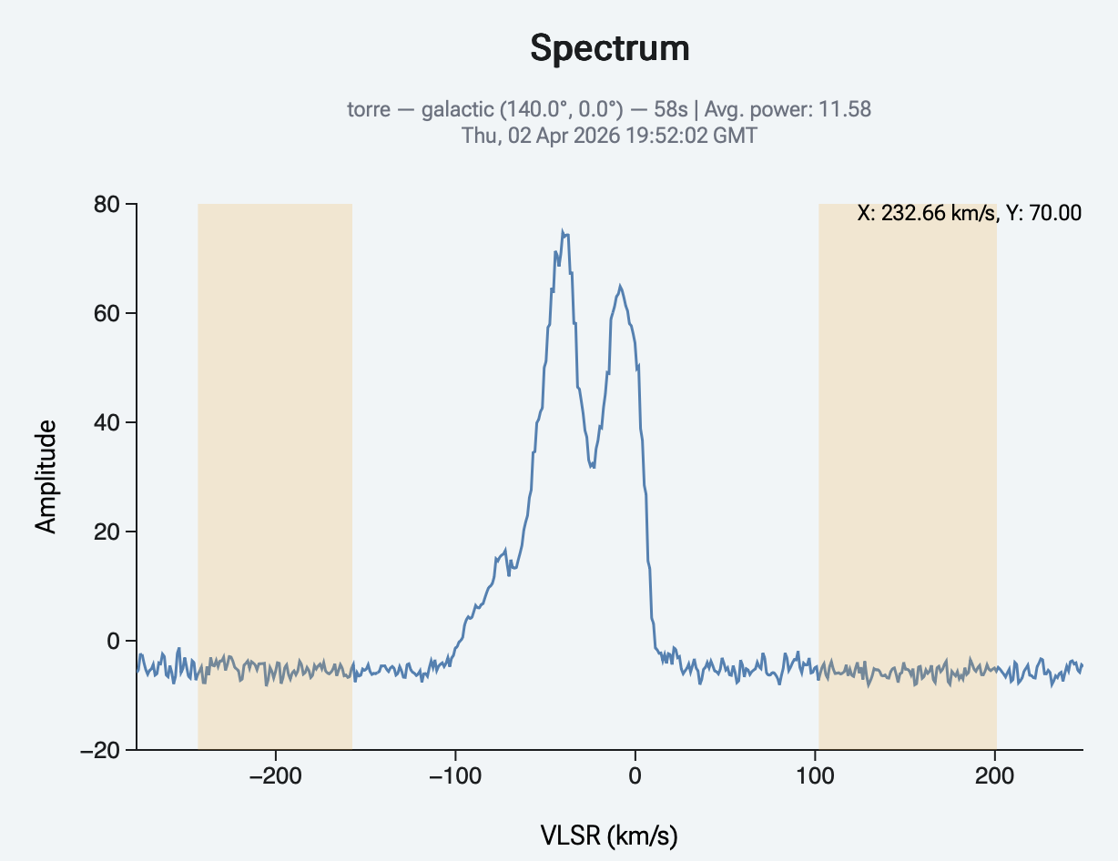
For galactic-coordinate observations, you can toggle the horizontal axis between frequency (MHz) and velocity (km/s) using the button below the chart. The velocity axis is in the Local Standard of Rest frame — SALSA applies the LSR correction automatically using the 21 cm hydrogen-line rest frequency, so values are directly comparable with published HI data. See HI experiment §1.5 for the details.
4. Observation archive
Go to Observation archive in the navigation bar to view all your saved observations. Each entry shows the start time, telescope, coordinate system, target position, and integration time. Click an observation to load its spectrum.
You can zoom into a region of the spectrum by drawing a box with the mouse. Double-click to reset the zoom.
4.1 Exporting data
Three export formats are available:
- PNG — An image of the corrected spectrum as displayed.
- CSV — Frequency and amplitude columns for use in a spreadsheet or analysis tool such as LibreOffice Calc or Matlab.
- FITS — The raw uncorrected spectrum in the standard astronomical FITS format, suitable for use with tools such as Astropy.
4.2 Spectral analysis tools
The archive page includes built-in tools for basic spectral analysis. Note that analysis results are not saved — take notes or export before leaving the page.
Baseline correction
Pick one or more frequency ranges that contain only noise (no signal), choose a polynomial order (linear or quadratic), then click Fit. A dashed orange curve shows the fitted polynomial. If it looks right, click Subtract to apply it; the spectrum flattens and the dashed curve disappears. If it doesn't, adjust the picks or the order and Fit again. Clear wipes the picked ranges, the pending fit, and undoes any previously applied subtraction — restoring the original spectrum.
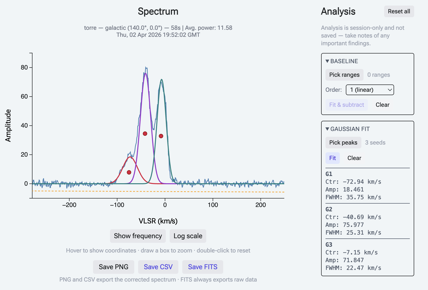
Gaussian fitting
After baseline correction, click on a peak in the spectrum to select it, then click Fit Gaussian. The fitted peak parameters (centre frequency, amplitude, width) are displayed.
Getting the fitter to converge on the right peaks can be tricky. For best results, click as close as possible to the very centre of each peak — both horizontally and vertically — during the peak-picking phase. See the example below.
5. Troubleshooting
Page layout is broken — items stacking vertically
SALSA's interface uses recent CSS features that older browsers don't support. You'll need at least Firefox 128, Chrome 111, or Safari 16.4 (or any later version). On older browsers, parts of the page that should appear side by side render stacked vertically instead — update your browser and reload.