GNSS satellite signal spectra
Based on earlier work by Grzegorz Klopotek, Onsala Space Observatory
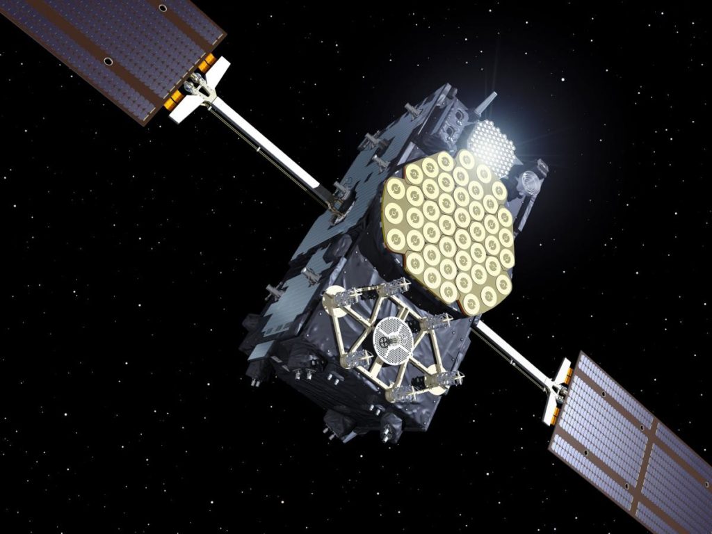
Every time you use a phone to navigate, it is relying on signals broadcast by satellites tens of thousands of kilometres overhead. These satellites — part of systems like GPS, Galileo, GLONASS, and BeiDou — continuously transmit radio signals in the L-band, around 1.2–1.6 GHz. With SALSA you can receive and inspect these signals directly, looking at how their radio spectra appear and comparing what different satellites and constellations look like.
This is a short, hands-on experiment. A few seconds of data per satellite is enough, and no complicated analysis is needed — the main result is visual: the spectra look different from one another, and that difference reflects real engineering choices made by each system.
Note: this guide focuses on the scientific background and what to look for in the spectra. Instructions for operating the telescope can be found in the User's manual.
1. Global Navigation Satellite Systems
1.1 The four constellations
A Global Navigation Satellite System (GNSS) is a network of satellites that continuously broadcast radio signals allowing receivers on the ground to determine their position with metre-level accuracy. Today there are four fully operational global systems:
| System | Operated by | Orbital altitude | Satellites | Key frequencies (MHz) |
|---|---|---|---|---|
| GPS | United States | ~20 200 km | ~31 | 1575.42 (L1), 1227.60 (L2), 1176.45 (L5) |
| Galileo | EU / ESA | ~23 200 km | ~24 | 1575.42 (E1), 1176.45 (E5a), 1207.14 (E5b), 1278.75 (E6) |
| GLONASS | Russia | ~19 100 km | ~24 | 1598–1606 (G1), 1243–1249 (G2) |
| BeiDou | China | ~21 500 km | ~35 | 1561.10 (B1), 1207.14 (B2), 1268.52 (B3) |
Each satellite orbits high enough that multiple satellites are visible simultaneously from any point on Earth. A receiver needs at minimum four satellites in view to solve for its three-dimensional position and clock offset.
1.2 GNSS signals and frequency bands
All GNSS satellites transmit in the L-band, roughly 1–2 GHz. This part of the radio spectrum was chosen because L-band signals pass through the atmosphere with minimal absorption, even in rain or cloud cover — unlike millimetre-wave frequencies that are strongly attenuated by water vapour. The signals do suffer a small delay in the ionosphere (the upper layer of atmosphere containing free electrons), but this effect is well-modelled and can be corrected using dual-frequency receivers.
The most commonly used band is L1/E1 at 1575.42 MHz, shared by GPS and Galileo. GLONASS uses a nearby but different frequency range for its G1 band (~1598–1606 MHz), and BeiDou's B1 signal sits at 1561.10 MHz. This means that SALSA, tuned to a single center frequency, will see signals from different constellations in different parts of the spectrum.
1.3 CDMA vs FDMA: two approaches to multiple access
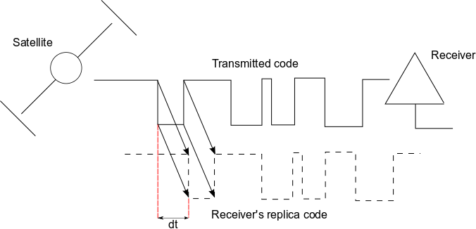
A key challenge in GNSS design is distinguishing signals from dozens of satellites all transmitting in the same frequency band simultaneously. Two different engineering solutions are used:
Code-Division Multiple Access (CDMA) — used by GPS, Galileo, and BeiDou. All satellites in a constellation transmit on the same frequency, but each uses a unique pseudorandom noise (PRN) code. Because these codes are nearly orthogonal, a receiver can separate them using correlation. From a radio telescope's perspective, all GPS satellites at L1 overlap spectrally — you cannot distinguish individual satellites by frequency.
Frequency-Division Multiple Access (FDMA) — used by legacy GLONASS. Each GLONASS satellite transmits on a slightly different frequency within the G1 band, separated by 562.5 kHz steps. This means individual GLONASS satellites are in principle separable by frequency with a narrowband receiver, though SALSA's 25 MHz bandwidth covers many simultaneously. Newer GLONASS satellites are adding CDMA capability as well.
1.4 Signal modulation and spectral shape
GNSS signals are not simple sinusoids — they are modulated with digital codes and navigation data, which spreads their energy across a range of frequencies and gives each signal a characteristic spectral shape:
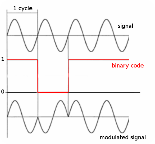
GPS L1 C/A (BPSK modulation): The civilian GPS L1 signal uses Binary Phase Shift Keying with a 1.023 MHz chip rate. This produces a sinc² spectrum: a central lobe about 2 MHz wide with smaller sidelobes on either side. With SALSA's 25 MHz bandwidth you can see the central lobe and the first few sidelobes clearly.
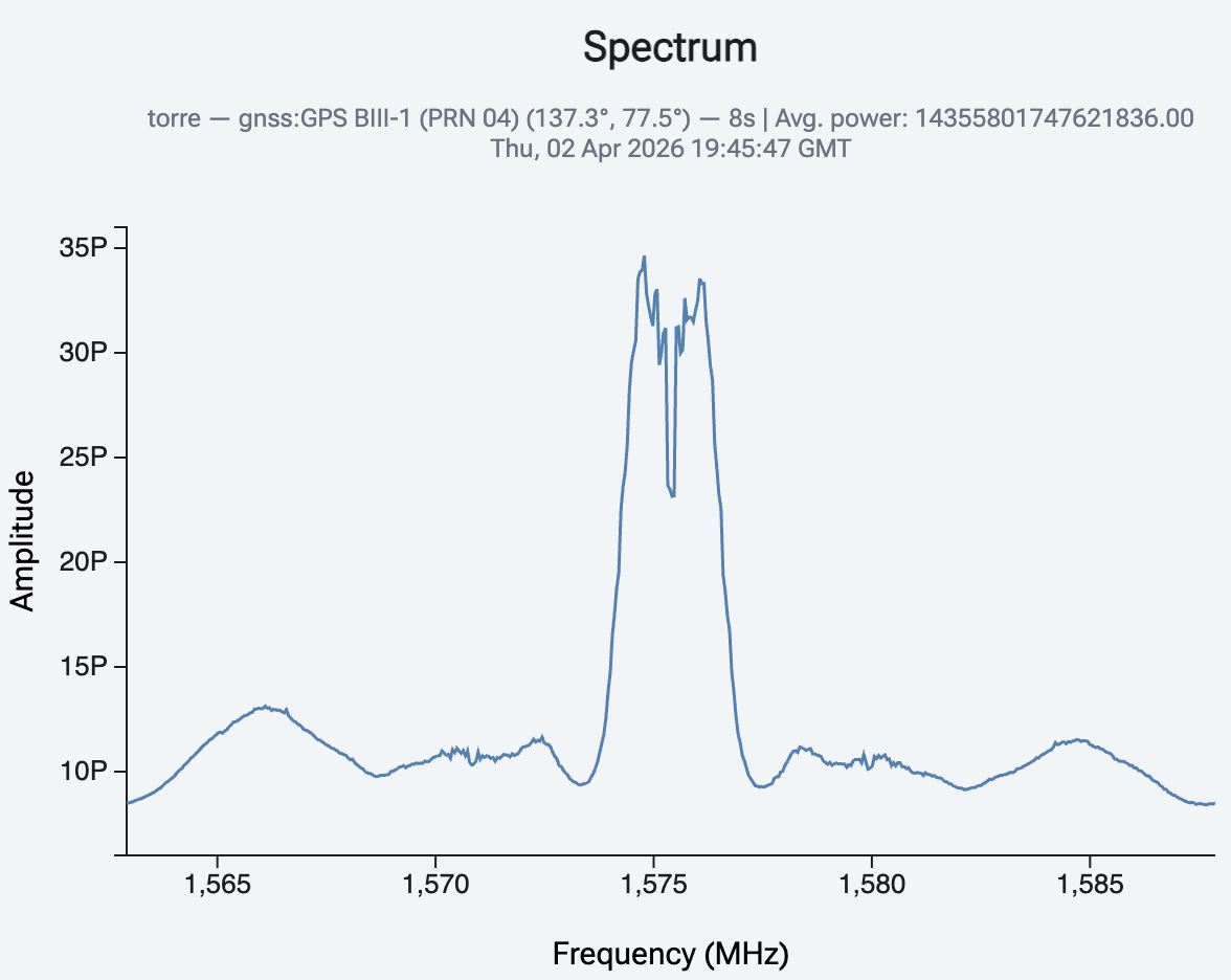
Galileo E1 (BOC modulation): Galileo's E1 signal uses Binary Offset Carrier modulation — BOC(1,1) — which shifts the signal energy away from the centre frequency, creating a characteristic double-humped (split-peak) spectrum. Even though GPS L1 and Galileo E1 share the same centre frequency of 1575.42 MHz, they look noticeably different in the spectrum.
GLONASS G1: GLONASS satellites use BPSK with a 0.511 MHz chip rate, and their individual center frequencies are spread across the G1 band. Each satellite contributes a narrower signal peak at its own frequency.
Detecting the difference between GPS and Galileo spectral shapes — both centred at 1575.42 MHz — is one of the most interesting things you can do with SALSA's GNSS mode.
2. Observing GNSS signals with SALSA
2.1 Selecting and tracking a satellite
- Open the observe page for your booked telescope.
- In the Target dropdown, select GNSS. The coordinate fields will be replaced by a satellite selector showing all satellites currently above the horizon, grouped by constellation (GPS, Galileo, GLONASS, BeiDou) with their current azimuth and elevation.
- Choose a satellite from the list. Try to pick one with an elevation well above the horizon — higher satellites give stronger, cleaner signals because the signal travels through less atmosphere and less ground interference. An elevation above 20° is a good starting point.
- Click Track. The telescope will slew to the satellite and follow it as it moves across the sky. Wait until the telescope has reached the target position before measuring.
The satellite list updates automatically. If you want to switch to a different satellite, click Stop, select a new satellite, and click Track again.
2.2 Receiver settings
When you select a satellite, SALSA automatically configures the receiver to sensible settings:
- Center frequency: set to the primary frequency for that satellite's constellation (e.g. 1575.42 MHz for GPS and Galileo, ~1602 MHz for GLONASS G1, 1561.10 MHz for BeiDou B1).
- Bandwidth: set to 25 MHz — wide enough to capture the full spectral shape of a GNSS signal including its sidelobes.
- Mode: set to Raw (total power), rather than the frequency-switched mode used for HI observations. GNSS signals are not spectral lines we need to subtract a reference from — we want to see the raw received power as a function of frequency.
You can check and adjust these settings under Advanced receiver settings if needed, but the defaults should work well for a first observation.
2.3 Taking a spectrum
Once the telescope is tracking, click Start to begin integrating. GNSS signals are strong — 1–2 seconds of integration is enough. You do not need long observations as you would for faint astronomical sources.
The resulting spectrum will appear in the chart. The horizontal axis shows frequency (or velocity, which you can toggle); the vertical axis shows uncalibrated antenna temperature in Kelvin. The values are relative, not absolute — you can compare spectra from different satellites to each other, but not directly to a calibrated flux density.
Try observing several satellites, one at a time, and note how their spectra compare.
3. Comparing satellite signals
3.1 GPS and Galileo at 1575 MHz
Observe a GPS satellite and a Galileo satellite, both tuned to 1575.42 MHz. Look carefully at the shape of the spectrum:
- A GPS satellite should show a broad central peak, widening smoothly from the centre — the sinc² shape of BPSK modulation.
- A Galileo satellite should show a distinctly different profile, with the energy split more towards the sides of the band — the double-humped shape of BOC(1,1) modulation.
This is the most striking comparison available with SALSA. Both signals are centred at exactly the same frequency, yet they are engineered to look different so that receivers can tell them apart. The BOC design was also chosen deliberately to make Galileo compatible with GPS (sharing the same band) while minimising interference between them.
Note that because GPS uses CDMA, all GPS satellites appear at the same frequency — if several GPS satellites are above the horizon, their signals add together in SALSA's beam. The same is true for Galileo. This is why switching between individual named GPS or Galileo satellites may not change the spectrum very much: the signal is a sum of all visible satellites in that constellation.
3.2 GLONASS: each satellite on its own frequency
Now observe a GLONASS satellite. The center frequency will be set automatically to that satellite's individual G1 frequency, which is close to 1602 MHz but varies by a small amount (each GLONASS satellite uses a different channel number, spaced 562.5 kHz apart). With SALSA's 25 MHz bandwidth you are seeing a slice of the G1 band.
The GLONASS signal will appear as a narrower peak, positioned at the satellite's own channel frequency rather than at a fixed constellation-wide value. Because each satellite is at a slightly different frequency (FDMA), GLONASS's spectrum within a 25 MHz window may contain contributions from multiple satellites at distinguishable positions — though at SALSA's spectral resolution they may overlap.
Compare the overall width and shape of the GLONASS spectrum to the GPS spectrum. The GLONASS signal uses a 0.511 MHz chip rate (compared to 1.023 MHz for GPS L1 C/A), so its central lobe is narrower.
3.3 How elevation affects signal strength
The strength of a received GNSS signal depends on the satellite's elevation above the horizon. There are two main reasons for this:
Free-space path loss: A satellite near the horizon is farther away than one directly overhead (the signal path through space is longer), so the signal arrives weaker. The path length to a satellite at 10° elevation is roughly 2–3 times longer than to a satellite at 90°, reducing received power by up to 10 dB.
Atmospheric and ground effects: A low-elevation satellite's signal passes through a much thicker slice of atmosphere, increasing absorption and scattering. Near the horizon the telescope may also receive additional noise from ground emission entering the beam sidelobes.
To see this effect: find the same satellite constellation at two different elevations (or compare two satellites of the same type at different elevations), and compare the peak amplitude of their spectra. You should see a clear difference in signal strength. For a fair comparison, make sure all other settings (integration time, bandwidth, gain) are identical.
Questions
- Observe a GPS satellite and a Galileo satellite. Can you see a difference in spectral shape? Describe what you observe and explain why the two signals look different.
- GPS satellites orbit at about 20 200 km altitude with a period of approximately 11 hours 58 minutes. Using the orbital period and the Earth's radius (6371 km), estimate the orbital speed of a GPS satellite. (Hint: the orbital circumference is 2π × (REarth + altitude).)
- Observe two satellites of the same type (e.g. two different GPS satellites) at different elevations. How does the signal strength change with elevation? Is the relationship what you would expect from simple geometry?
- The free-space path loss at frequency f and distance R is LFS = (4πRf/c)². Calculate the path loss in dB for a GPS L1 signal (1575.42 MHz) at a satellite distance of 25 000 km. How would this compare to a signal at 10 GHz at the same distance?
- Look at the GLONASS spectrum. Can you tell that GLONASS uses a different multiple-access scheme than GPS from the appearance of the spectrum? What would you expect to see if you tracked two different GLONASS satellites with similar settings?
- Can you think of any sources of radio interference in the 1575 MHz band that might affect the SALSA observations? How might this appear in the spectrum?