Mapping the Milky Way
Written by Cathy Horellou, Daniel Johansson & Eskil Varenius
In this document we first review some properties of the Milky Way, starting by describing the Galactic coordinate system and the geometry of a rotating disk. Then, we describe how to use data from SALSA to understand how fast gas rotates at different distances from the galactic center, i.e. how to make a rotation curve. Finally, we use additional measurements, and our knowledge of the kinematics, to make a map of the spiral arms.
Note: this document is focused on the scientific interpretation. Instructions for operating the SALSA telescope can be found on the Support & documentation page.
1. Welcome to the Galaxy
Looking up on a clear, dark night, our eyes are able to discern a luminous band stretching across the sky. Observe it with binoculars or a small telescope and you will discover, like Galileo in 1609, that it is made up of a myriad of stars. This is the Milky Way: our own Galaxy, as it appears from Earth. It contains about a hundred billions of stars, and our Sun is just one of them. There are many other galaxies in the universe. We also refer to the Milky Way as just the Galaxy.
It took astronomers a long time to figure out what the Galaxy really looks like. One would like to be able to embark on a spaceship and see the Galaxy from outside. Unfortunately, traveling in and around the Galaxy is (and will always be) out of the question because of the huge distances. We are condemned to observe the Galaxy from the vicinity of the Sun.
Observations of the Galaxy, as well as of other galaxies, using both optical and radio telescopes, have helped unveil the structure of our galaxy. Today, astronomers think they have good knowledge of how the stars and gas clouds are distributed. Our galaxy seems to be a thin disk of stars and gas, which are distributed in a spiral pattern.
But a new mystery has arisen: that of the so-called dark matter. Most of the mass of our galaxy seems to be in the form of dark matter, a mysterious component that has, so far, escaped all means of identification. Its existence has been inferred only indirectly. Imagine a couple of dancers, in a dark room. The man is black, dressed in black clothes, and the woman wears a fluorescent dress. You can't see the man. But from the motion of the woman dancer, you can infer his presence: somebody must be holding onto her, otherwise, with such speed, she would simply fly away! Similarly, the stars and the gas in our galaxy rotate too fast, compared to the amount of mass observed. There must therefore be more matter, invisible to our eyes and to the most sensitive instruments, but which, through the force of gravity, holds the stars together in our galaxy and prevents them from flying away. The key argument in favor of the existence of dark matter comes from the measured velocities in the outer part of our galaxy. Radio measurements of the type described in this document have played an important role in revealing the presence of dark matter in the Milky Way. But what dark matter really is remains an open question.
1.1 Our place in the Milky Way
Our star, the Sun, is located in the outer part of the Galaxy, at a distance of about 8.5 kpc1 (about 25 000 light years2) from the Galactic center. Most of the stars and the gas lie in a thin disk and rotate around the Galactic center. The Sun has a circular speed of about 220 km/s, and performs a full revolution around the center of the Galaxy in about 240 million years.
1 1 kpc = 1 kiloparsec = 103 pc; 1 parallax-second
(parsec, pc) = 3.086·1016 m. A parsec is the distance from which
the radius of Earth's orbit subtends an angle of 1″ (1 arcsec).
2 1 light year (ly) = 9.4605·1015 m.
1.2 Galactic coordinates: longitude and latitude
To describe the position of a star or a gas cloud in the Galaxy, it is convenient to use the so-called Galactic coordinate system, (l, b), where l is the Galactic longitude and b the Galactic latitude. The Galactic coordinate system is centered on the Sun. b = 0 corresponds to the Galactic plane. The direction b = 90° is called the North Galactic Pole. The longitude l is measured counterclockwise from the direction from the Sun toward the Galactic center. The Galactic center thus has the coordinates (l = 0, b = 0). There is, in fact, something very special at the Galactic center: a very large concentration of mass in the form of a black hole containing approximately three million times the mass of the Sun. Surrounding it is a brilliant source of radio waves and X-rays called Sagittarius A*.
The Galaxy has been divided into four quadrants, labeled by Roman numbers:
| Quadrant | Range |
|---|---|
| I | 0° < l < 90° |
| II | 90° < l < 180° |
| III | 180° < l < 270° |
| IV | 270° < l < 360° |
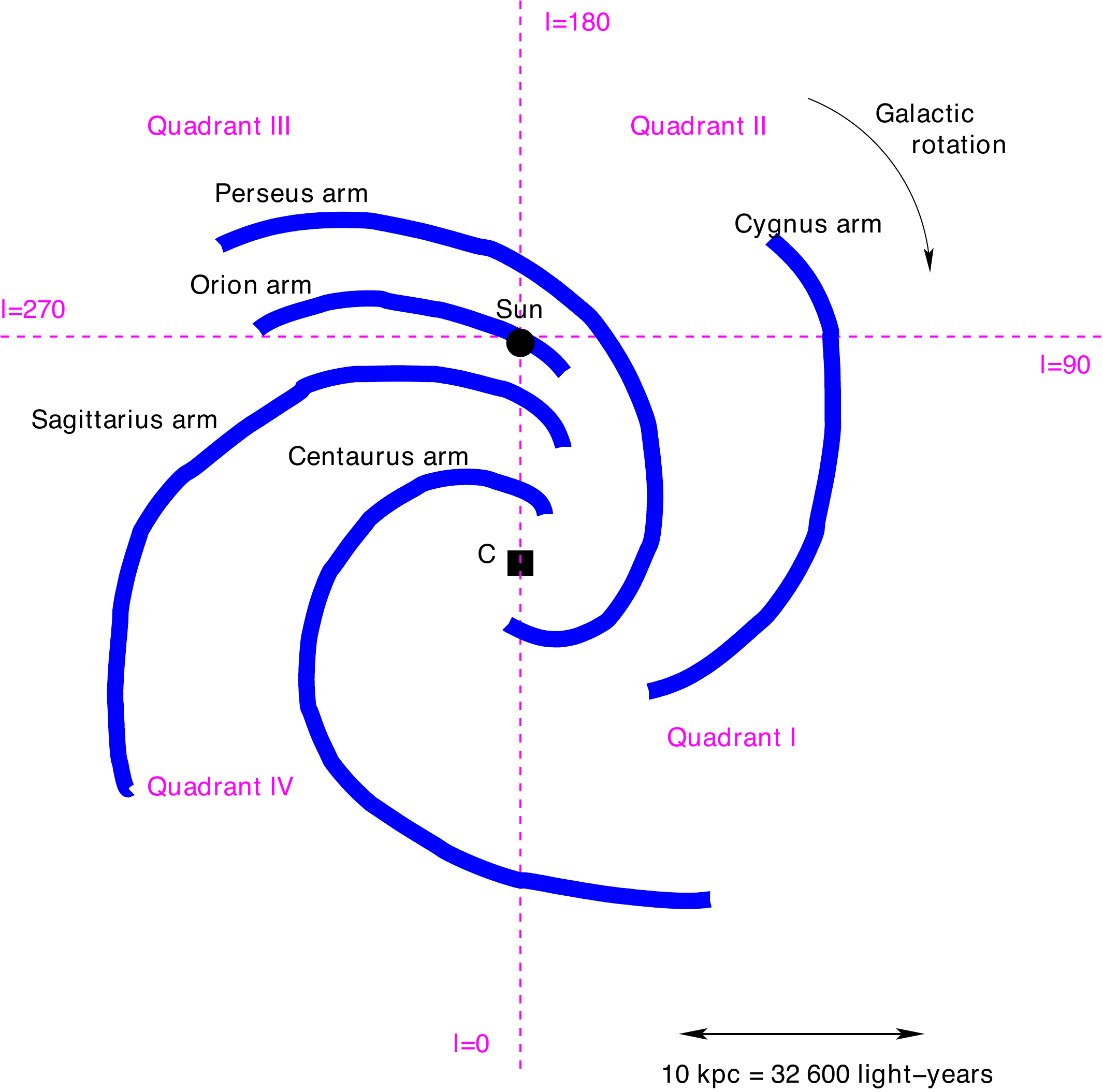
In Quadrants I and IV we observe mainly the inner part of our Galaxy. Quadrants II and III contain material lying at galacto-centric radii which are always larger than the Solar radius (the radius of the orbit of the Sun around the Galactic center).
1.3 Radio emission from atomic hydrogen
Most of the gas in the Galaxy is atomic hydrogen (H). H is the simplest atom: it has only one proton and one electron. Atomic hydrogen emits a radio line at a wavelength λ = 21 cm (or a frequency f = c/λ = 1420 MHz, where c ≅ 300 000 km/s is the speed of light). This is the signal we want to detect.
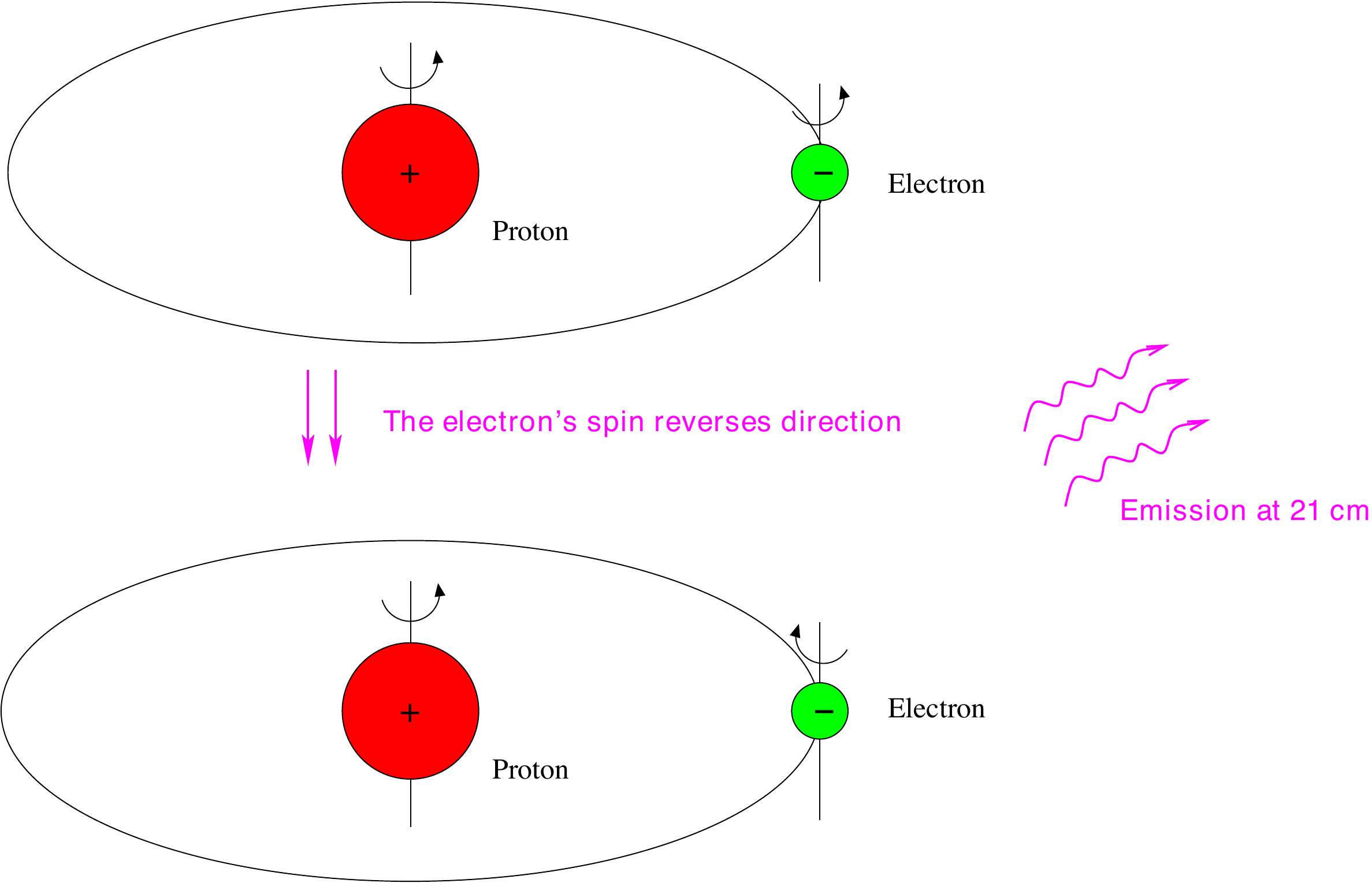
The 21 cm hydrogen signal is emitted when the electron's spin flips from being parallel to being antiparallel with the proton's spin, bringing the atom to a lower energy state. Although this happens spontaneously only about once every ten million years for a given hydrogen atom, the enormous quantity of hydrogen in the Milky Way makes the 21 cm line detectable. The line was predicted by the Dutch astronomer H.C. van de Hulst in 1945, who determined its frequency theoretically. The line was observed for the first time in 1951 by three groups, in the U.S.A., in the Netherlands and in Australia (see Appendix B).
1.4 The Doppler effect
By observing radio emission from hydrogen, we can learn about the motion of the hydrogen gas clouds in our Galaxy. Indeed, it is possible to relate the observed frequency of the signal to the velocity of the emitting gas, thanks to the so-called Doppler effect.
This effect, named after the Austrian physicist Christian Johann Doppler (1803–1853), is also present in our everyday life; for example if you are standing still in the street and an ambulance approaches you, it appears as if the pitch of the ambulance's siren increases. Similarly, when the ambulance is receding, the pitch of the siren decreases. Because sound waves travel through a medium (the air), when the ambulance is approaching the waves will be 'squeezed' together by the forward motion. Shorter wavelengths mean higher frequency, and thus the pitch of the siren increases. This effect, that the frequency of the waves changes because of motion, is the Doppler effect.
We can use the Doppler effect to relate the frequency we observe to the velocity of the emitting hydrogen gas cloud, but to do so we need a formula. We chose to omit the rather long derivation and just state the important relation between the observed frequency shift and the velocity:
where:
- Δf = f − f₀ is the frequency shift,
- f is the observed frequency,
- f₀ is the rest frequency of the line we are observing,
- v is the velocity: > 0 if the object is receding, < 0 if it is approaching.
To observe hydrogen emission from gas clouds in the Galaxy we tune the receiver of our radio telescope to record frequencies near the rest frequency of the hydrogen line, i.e. the frequency we would measure if there was no relative motion. Clouds with different velocities will then appear at different frequencies. The frequency will be shifted up or down when the signal reaches us, depending on whether the gas cloud that we observe is approaching us or receding from us.
1.5 The Local Standard of Rest
The velocity computed from the Doppler formula above is relative to the telescope — but the telescope is not stationary. Earth rotates, orbits the Sun, and the Sun itself moves through the Galaxy. If you observe the same hydrogen cloud at different times of day or year, the telescope-frame velocity changes simply because the telescope's motion has changed, even though the cloud has not.
To make measurements comparable across different times and observing sites, astronomers convert this telescope-frame velocity into the Local Standard of Rest (LSR) frame: a notional frame at the Sun's position with the Sun's peculiar motion removed. In the LSR frame, gas clouds in the Galaxy have well-defined velocities that match published HI maps and rotation-curve measurements.
SALSA computes and applies this correction automatically whenever you observe a galactic-coordinate target, using the 21 cm hydrogen-line rest frequency (1420.405 MHz) as the reference. The velocity axis on the spectrum chart is therefore in the LSR frame for galactic targets — directly comparable with literature values without further correction. For non-galactic targets (Sun, satellites), no LSR correction is computed.
For more on the LSR frame and how it is defined, see Wikipedia: Local standard of rest.
2. The structure and kinematics of the Milky Way
In this chapter we describe how SALSA can be used to measure the structure and kinematics of the Milky Way. First we explain how to measure the rotation curve, i.e. the rotational speed of the gas at different distances from the galactic center. Then we build on these results to make a map of the spiral arms.
2.1 The rotation curve of the Milky Way
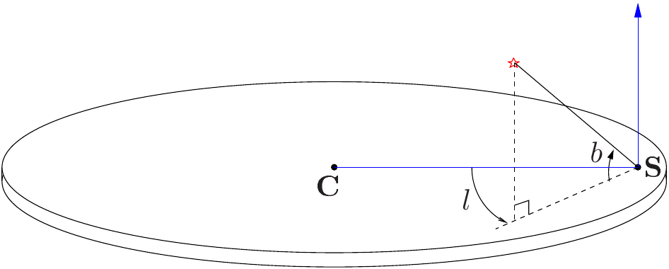
A rotation curve is a function which describes the rotational speed of the galaxy at different distances from the center, usually denoted V(R). To construct a rotation curve we first need to understand how the velocity we measure (through Doppler shift) is related to the movement of gas clouds in the Milky Way. Let us imagine that we point our radio telescope towards a gas cloud in the Galaxy, i.e. we observe along the line of sight in Fig. 2.1. For future reference we list some variables used in this figure:
| Symbol | Meaning |
|---|---|
| V₀ | Sun's velocity around the Galactic center, i.e. 220 km/s |
| R₀ | Distance of the Sun to the Galactic center, i.e. 8.5 kpc |
| l | Galactic longitude of observation |
| V | Velocity of a cloud of gas |
| R | Cloud's distance to the Galactic center |
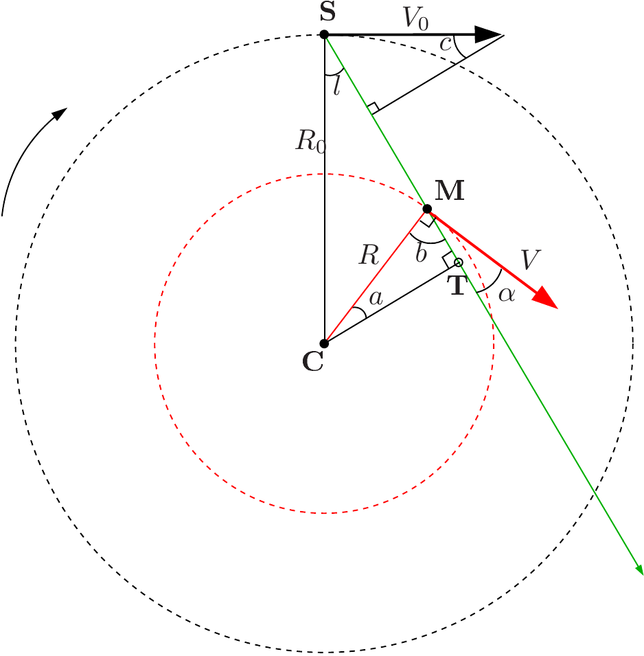
There may be many clouds in this direction, but for the purpose of this derivation we only care about a single cloud located at position M in Fig. 2.1. Since both the Sun and the cloud are moving, we do not measure the cloud velocity directly. Instead, we measure the relative velocity, Vr, between us and the cloud, projected on the line-of-sight. Using the angles in Fig. 2.1 we can write this down as
For this expression to be useful we need to relate the angles to the galactic coordinates we discussed in Sect. 1.2. We know that the sum of angles in the upper right triangle must be 180°, which means that we can relate the angle c to galactic longitude l as
We now want to relate also the angle α to the longitude l. We note that the angle between V and R is 90° and can be written as the sum of a and α, i.e. 90° = b + α. From the triangle CMT we also note that b = 90° − a. Put together we get
Looking at the triangles CST and CMT we find that the distance between the Galactic Center (C) and the tangential point (T) can be expressed in two different ways:
Using equations 2.2, 2.3, and 2.4 we can now re-write equation 2.1 as
This equation is valid for all longitudes l. However, measuring Vr alone for any given l is not enough to solve this equation to derive both V and R. A solution is to restrict the range of possible l to the first quadrant, and using only the maximum velocity detected in our calculations. We now explain how this simplifies the problem.
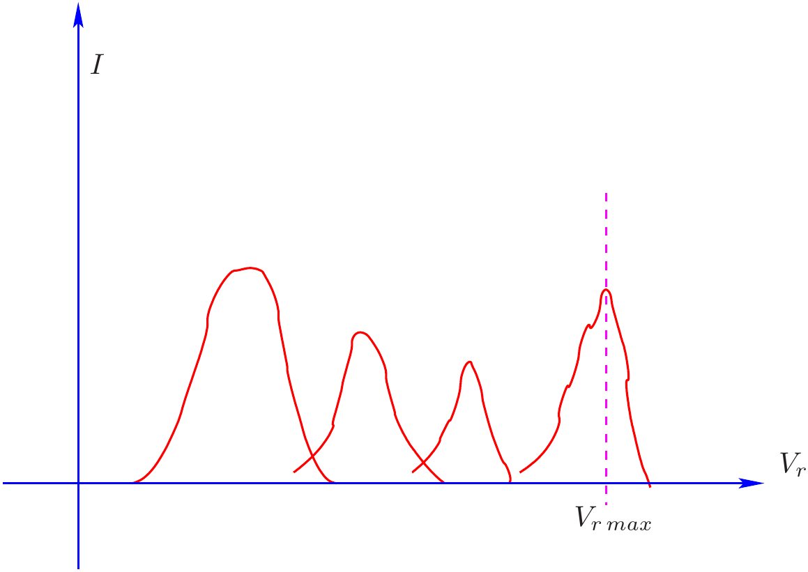
In any given direction we may observe emission from multiple clouds at once. Since the clouds move with different relative velocities, we measure multiple components in the spectrum, as illustrated in Fig. 2.2. We now assume that clouds at larger distances from the center move with equal or lower speed than clouds closer to the center, as expected from standard Keplerian motion (see Appendix A). In this case, the largest velocity component, Vr,max, comes from the cloud at the tangential point (T), since the maximum possible projected velocity happens when the projection angle is 0. For a cloud at the tangent point we see from Fig. 2.1 that the cloud location is given by
This simplifies equation 2.5 so that, at the tangential point, we have:
We may now use SALSA to measure Vr,max at different l in the first quadrant. Using equations 2.6 and 2.7 we may then calculate the rotation curve V(R). It is reasonable to assume the measured rotation curve to be valid also in the other three quadrants.
2.1.1 Measure the rotation curve with SALSA
After reading the previous section you should have an idea about how to measure the rotation curve of the Milky Way using SALSA. Instructions for how to operate the telescope are given on the Support & documentation page. Once you have obtained spectra at a few selected longitudes, extract the maximum velocity of each spectrum and plot the rotation curve. The simplest way is to use the cursor to inspect the spectrum directly in the control program, but you can also use more advanced tools such as Matlab.
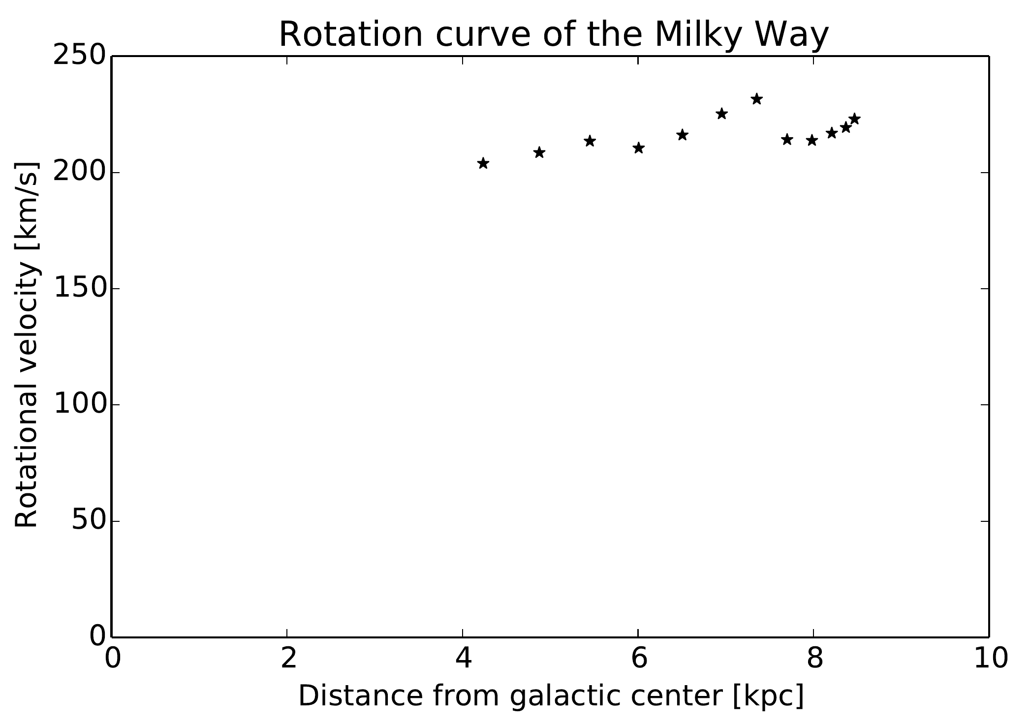
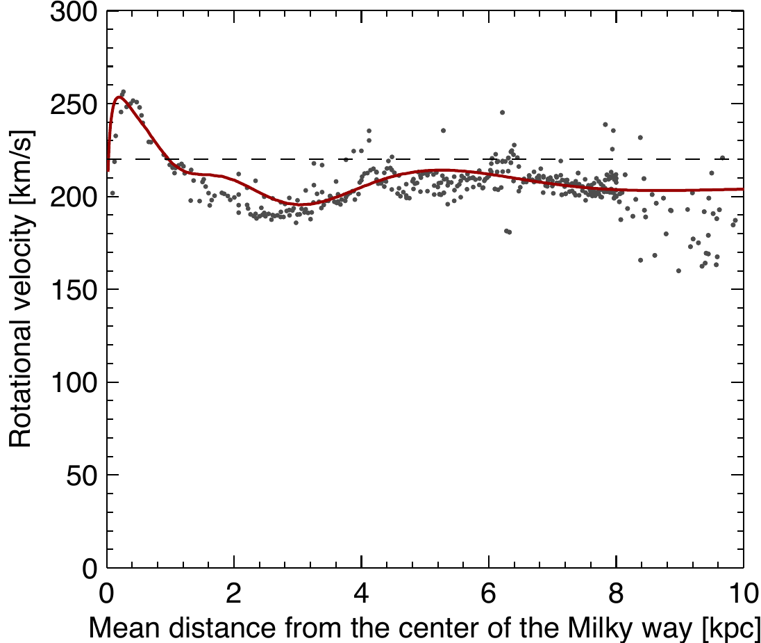
To make the final plot of the rotation curve you may use your favourite plotting program. A simple free solution is to use the Excel-like program LibreOffice Calc, where you can put your calculated values of V and R in a spreadsheet and then use the xy-chart to plot the data. Your final plot should look similar to Fig. 2.3. Note that the rotation curve is almost flat! This is an indirect evidence for dark matter in our galaxy. You may also want to compare with the results in Appendix A, and compare your measured spectra with reference data from large-scale HI surveys (see Appendix C).
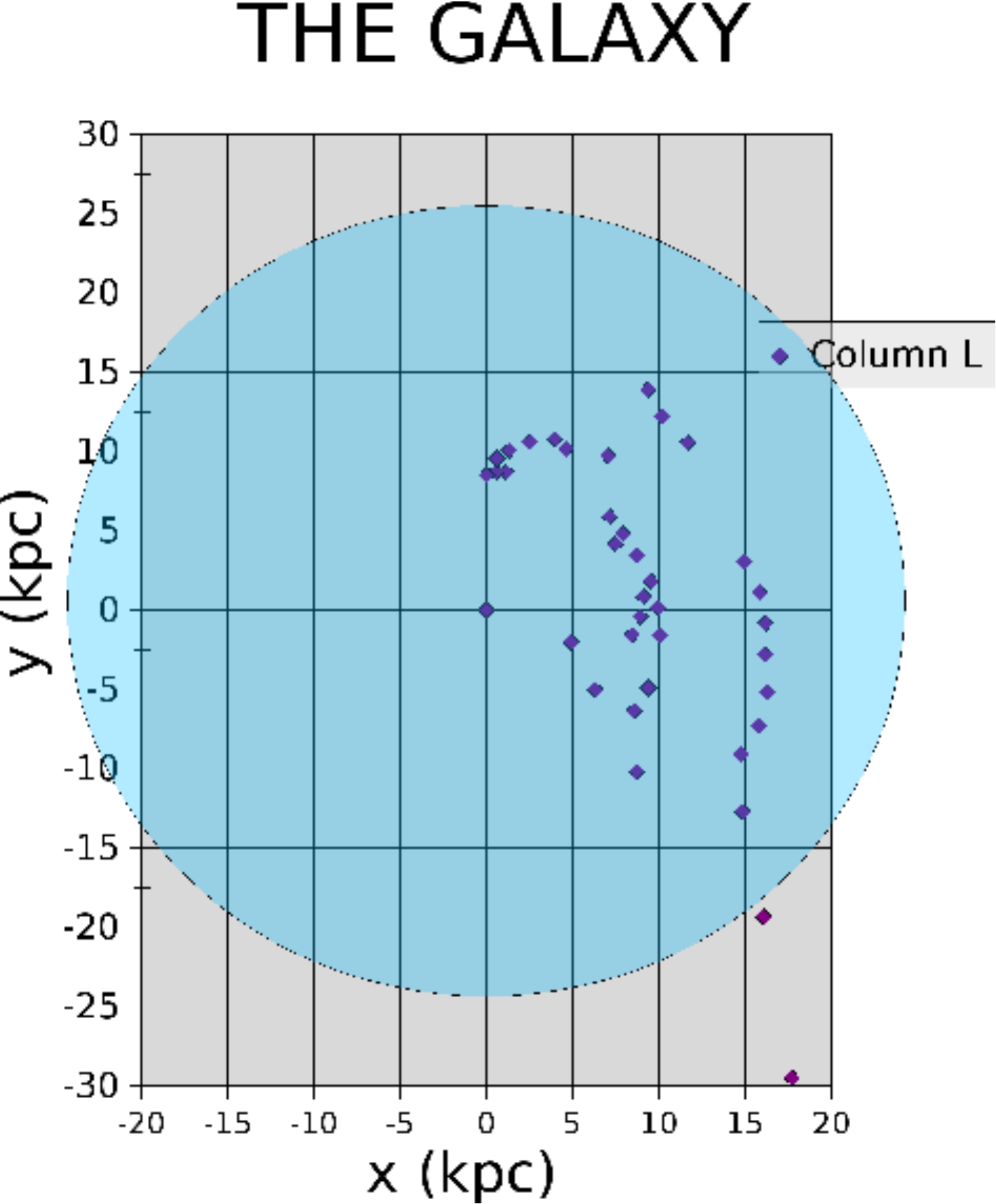
2.2 Mapping the Milky Way
Now we would like to find out where the HI gas that we have detected is located. Let us therefore return to equation 2.5. When finding the rotation curve, we used only the maximum velocity component in the spectrum, and assumed that it came from gas at the tangential point. This assumption made it possible to solve equation 2.5 in the first quadrant. Now, we shall use all the velocity components that we see in our spectra, and we want to be able to map in all observable directions, not only in the first quadrant. We can now use our knowledge about the rotation curve obtained in Sect. 2.1.1. Motivated by the shape of our measured rotation curve we now assume that the gas in our Milky Way obeys differential rotation, i.e. the rotational speed is constant with radius and is the same as the rotational speed of the Sun, i.e.
With this assumption, equation 2.5 simplifies to
This equation can be re-written as an expression for the cloud distance R as a function of known (or observable, in the case of Vr) quantities:
Now we would like to make a map of the Milky Way and place the position of the cloud that we have detected. From our measurement of the radial velocity Vr we have just calculated the distance of the cloud to the Galactic center, R, and we know in which direction we have observed (the Galactic longitude l).
Please note that if you observe in Quadrants II or III, then the position of the emitting gas clouds can be determined uniquely. But, if observing in Quadrants I or IV, there may be two possible locations corresponding to given values of l and R: closer to us than the tangential point T (the actual point M on the figure), or farther away, at the intersection of the ST line and the inner circle (see Fig. 2.1). You may want to make a drawing to convince yourself that this is true.
This distance ambiguity can also be shown mathematically. Let r denote the distance from the Sun to the cloud, i.e. the distance between the points S and M in Fig. 2.1. Using the law of cosines on the triangle CSM we obtain the following relation:
This is a second-order equation in r, which has two possible solutions. If we denote these solutions r = r+ and r = r−, we can write the solutions as
We note a couple of things regarding the above equation. For some data points one finds one positive and one negative solution for r. The negative solution is not meaningful (it would mean on the other side of the Sun) and should be discarded. In Quadrants II or III, R is always larger than R₀ and cos l < 0, meaning there is one and only one positive solution, r+. In Quadrants I or IV, there may be two positive, and therefore possible, solutions. In cases with two possible solutions it is not possible to determine which one is the correct one without additional observations. To resolve this ambiguity, one can observe again towards the same galactic longitude but towards a small (a few degrees) non-zero galactic latitude. If the ambiguous cloud is far away, it should no longer be seen. If the cloud is close, it should still appear even if observing slightly out of the plane. Some experimenting may be necessary here to find out the appropriate galactic latitude.
2.2.1 Converting from r and l to Cartesian coordinates
For plotting it may be inconvenient to use the coordinates r (distance to cloud from the Sun) and l (galactic longitude) to describe the cloud positions. Instead it is usually more convenient to transform to a Cartesian system of perpendicular coordinates x and y. To convert to x–y coordinates we need to relate them to r and l.
You are probably familiar with polar coordinates, usually defined as
y = r sin θ (2.13)
where r is the distance from the origin and θ is the rotation angle, and x and y are Cartesian coordinates.
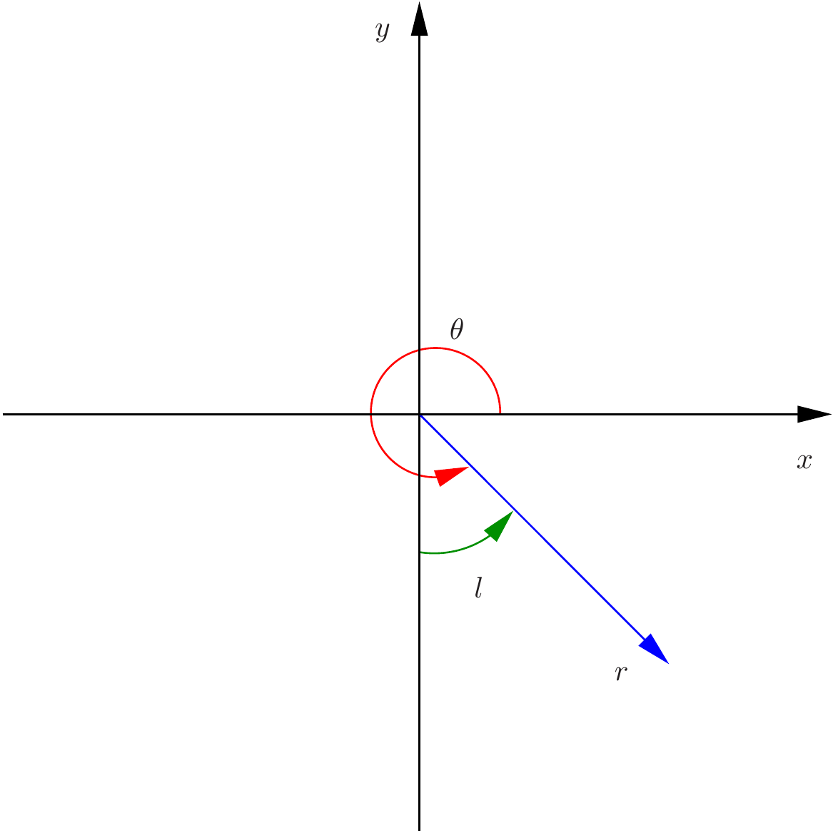
It is clear that polar coordinates are very similar to our r, l-system. We find that θ = 270° + l, or θ = l − 90°. This means that we can convert our positions given as r, l to Cartesian x–y coordinates by:
y = r sin(l − 90°) (2.14)
This format is usually the most convenient to plot the positions. Note that this will show the map with Earth in the center, at position (0, 0). If you instead want the Galactic center to be at (0, 0), add R₀ to the y-coordinate of each point.
2.2.2 Make a map with SALSA
After reading the previous section you should have an idea about how to construct a map from measured velocities. The measurements are done in the same way as you did in Sect. 2.1.1, but now you do not have to measure in the first quadrant. Also, you should extract all velocity components in your spectra, not only the maximum one. Again, instructions for how to operate the telescope are given on the Support & documentation page. The simplest way to obtain velocities from a spectrum is to use the cursor to inspect the spectrum directly in the control program, but you can also use more advanced tools such as Matlab.
Once you have a list of measured velocities for multiple longitudes you can use equation 2.12 to find the position of the clouds. Note that observations in Quadrants I or IV may need additional observations to resolve possible distance ambiguities, as discussed in the previous section.
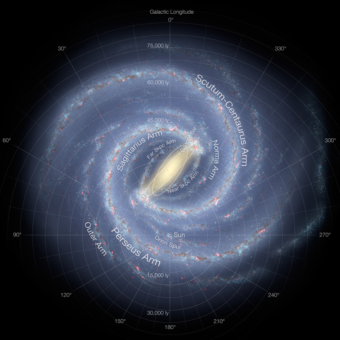
To make the final map you may use your favourite plotting program. Again, a simple free solution is to use the Excel-like program LibreOffice Calc, where you can put your calculated positions (x, y) in a spreadsheet and then use the xy-chart to plot the data. Your final map may look similar to Fig. 2.5, although it will depend on in which directions you have been observing. You may also want to compare with the cover image at the top of this page, and to verify your spectra against professional survey data (see Appendix C).
Appendices
A. Rotation curves
A rotation curve shows the circular velocity as a function of radius. We discuss here three different types of rotation curves.
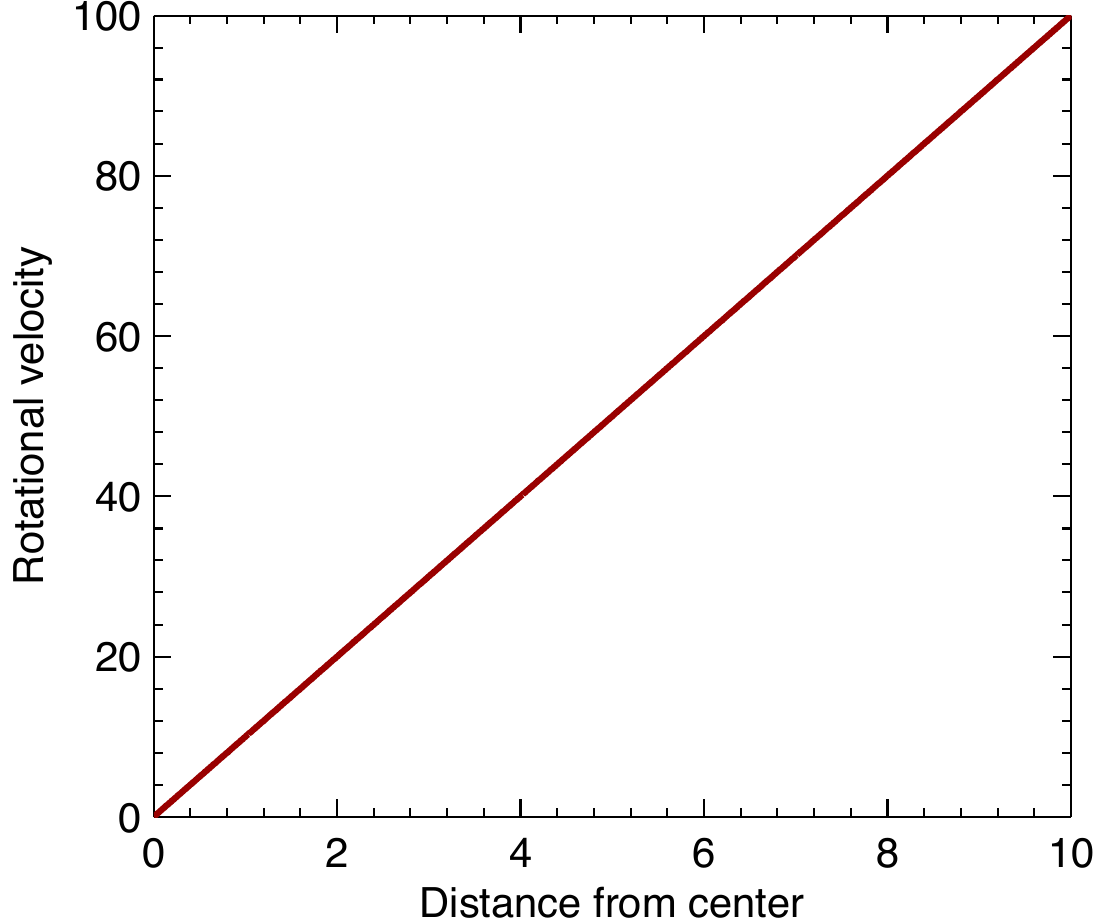
A.1 Solid-body rotation
Think of a solid turntable, or a rotating DVD-disc. It rotates with a constant angular speed Ω = V/R = constant. The circular velocity is therefore proportional to the radius:
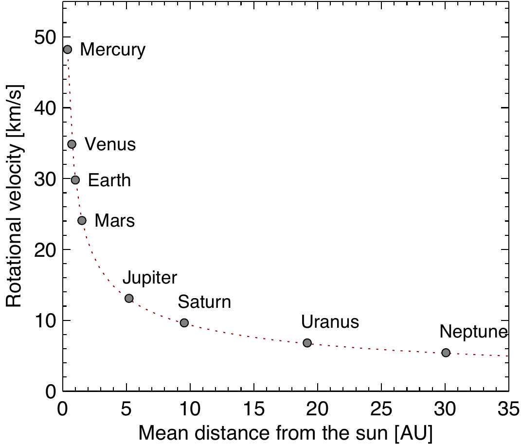
A.2 Keplerian rotation: the Solar system
In the Solar system, the planets have a negligible mass compared to the mass of the Sun. Therefore the center of mass of the Solar system is very close to the center of the Sun. The centrifugal acceleration from the planet's circular velocities counterbalances the gravitational acceleration:
where M is the mass and G the gravitational constant. The rotation curve is said to be Keplerian, and the velocities decrease with increasing radius:
A.3 The rotation curve of a spiral galaxy
Similarly, the rotation curve of a galaxy V(R) shows the circular velocity as a function of galacto-centric radius. In contrast to the rotation curve of systems like the Solar system with a large central mass, most galaxies exhibit flat rotation curves, that is, V(R) doesn't depend on R beyond a certain radius:
The angular velocity varies as Ω ∝ 1/R. Matter near the center rotates with a larger angular speed than matter farther away.
At large radii, the velocities are significantly larger than in the Keplerian case, and this is an indication of the existence of additional matter at large radii. This is an indirect way to show the existence of dark matter in galaxies.
B. Early history of 21 cm line observations
The story of the discovery of the 21 cm line of hydrogen is a fascinating one because it began during the Second World War, when international scientific contacts were disrupted and some scientists were struggling to carry out research.
In 1944, H.C. van de Hulst, a student in Holland, scientifically isolated because of the Nazi occupation of his country, presented a paper at a colloquium in Leiden in which he showed that the hyperfine levels of the ground state of the hydrogen atom produce a spectral line at a wavelength of about 21 cm, and that it could be detectable in the Galaxy. An article was published in a Dutch journal (Bakker and van de Hulst 1945).
After the war, efforts were made in several countries to design and construct equipment to detect the spectral line. It was first observed in the United States by Ewen and Purcell on 21 March 1951; in May the same year, it was observed by Muller and Oort (1951) in Holland. Both papers were published in the same issue of the journal Nature. Within two months Christiansen and Hindman (1952) in Australia had detected the line.
The first systematic investigation of HI in the Galaxy was made in Holland by van de Hulst, Muller, and Oort (1954). The Dutch group used a reflector from a German radar receiver of the "Great Würzburg" type, 7.5 m in diameter. The beamwidth at λ21 cm was 1°.9 in the horizontal direction and 2°.7 in the vertical direction.
Christiansen and Hindman used a section of a paraboloidal reflector, with a beamwidth of about 2°.
C. Comparative HI data
For comparison with your SALSA observations, the Bonn University HI profile server provides HI spectra from the GASS and LAB surveys covering the full sky. When querying, set the effective beam size to 6° for results comparable to SALSA.
Bibliography
- Bakker, C.J., van de Hulst, H.C., 1945, Nederl. Tijds. v. Natuurkunde 11, 201. (Bakker, "Ontvangst [reception] der radiogolven"; van de Hulst, "Herkomst [origin] der radiogolven".)
- Burton, W.B., in Galactic and Extragalactic Radio Astronomy, 1988, Verschuur G.L., Kellermann, K.I. (eds.), Springer-Verlag.
- Cohen-Tannoudji, C., Diu, B., Laloë, F., 1986, Quantum Mechanics, Vol. 1 and 2, Wiley-VCH. (See Chapters VII.C and XII.D about the hydrogen atom.)
- Ewen, H.I., Purcell, E.M., 1951, Nature 168, 356, "Radiation from galactic hydrogen at 1420 Mc/s".
- Hulst, H.C. van de, Muller, C.A., Oort, J.H., 1954, B.A.N. 12, 117, "The spiral structure of the outer part of the galactic system derived from the hydrogen emission at 21-cm wavelength".
- Lang, K.R., 1999, Astrophysical Formulae, Volume II: Space, Time, Matter, and Cosmology, Springer-Verlag.
- Muller, C.A., Oort, J.H., 1951, Nature 168, 357, "The interstellar hydrogen line at 1420 Mc/s, and an estimate of galactic rotation".
- Peebles, P.J.E., 1992, Quantum Mechanics, Princeton University Press, p. 273–303.
- Rigden, J.S., 2003, Hydrogen, The Essential Element, chap. 7, Harvard University Press.
- Shklovsky, I.S., 1960, Cosmic Radio Waves, translated by R.B. Rodman and C.M. Varsavsky, Harvard University Press.
- Sofue, Y., Honma, M., Omodaka, T. (2009). "Unified Rotation Curve of the Galaxy — Decomposition into de Vaucouleurs Bulge, Disk, Dark Halo, and the 9-kpc Rotation Dip." PASJ, 61:227.